Assignment 1

Background Coding

library(tidyverse)

df_pk6_2024 <- read_csv(here::here("posts/html/mm_first_story/School_Expenditures_by_Spending_Category_20260208.csv"))

names(df_pk6_2024)

 [1] "SY"             "DIST_CODE"      "DIST_NAME"      "ORG_CODE"      
 [5] "ORG_NAME"       "GRADES_SERVED"  "IND_CAT"        "IND_SUBCAT"    
 [9] "IND_VALUE"      "IND_VALUE_TYPE"

nrow(df_pk6_2024)

[1] 16112

Citations: tidyr 1.3.2 (https://tidyr.tidyverse.org/articles/pivot.html) was used for information on pivoting a data set

Filtering the data to only the MCAS Performance and District Reported Expenses

df_analysis_long <- df_pk6_2024 %>%
  filter(
    (IND_CAT == "Sub-Total A" & IND_SUBCAT == "District Non-Instructional Expenditures") |
    (IND_CAT == "Sub-Total B" & IND_SUBCAT == "District-Level Instructional Expenditures") |
    (IND_CAT == "Sub-Total C" & IND_SUBCAT == "School-Reported Instructional Expenditures") |
    (IND_CAT == "MCAS Performance" & IND_SUBCAT == "Math Grades 3-8 % Meets or Exceeds")
  )

Pivoting wider so that each school is one row

analysis_df <- df_analysis_long %>%
  select(DIST_CODE, DIST_NAME, IND_SUBCAT, IND_VALUE) %>%
  pivot_wider(
    names_from = IND_SUBCAT,
    values_from = IND_VALUE
  )

Mutating the data so that it is all read as numbers

clean_numeric <- function(x) {
  x <- gsub(",", "", x)           # remove commas
  x <- str_trim(x)                 # remove leading/trailing spaces
  x[x == "–" | x == "N/A"] <- NA  # treat common placeholders as NA
  as.numeric(x)                    # convert to numeric
}

analysis_df <- analysis_df %>%
  mutate(
    `District Non-Instructional Expenditures` = clean_numeric(`District Non-Instructional Expenditures`),
    `District-Level Instructional Expenditures` = clean_numeric(`District-Level Instructional Expenditures`),
    `School-Reported Instructional Expenditures` = clean_numeric(`School-Reported Instructional Expenditures`),
    `Math Grades 3-8 % Meets or Exceeds` = clean_numeric(`Math Grades 3-8 % Meets or Exceeds`)
  ) %>%
  drop_na(
    `District Non-Instructional Expenditures`,
    `District-Level Instructional Expenditures`,
    `School-Reported Instructional Expenditures`,
    `Math Grades 3-8 % Meets or Exceeds`
  )

Cleaning of the Model did not respond to simplue mutations likly becasue of missing data and thus that was dealt with seperatly.

model <- lm(
  `Math Grades 3-8 % Meets or Exceeds` ~ 
    `School-Reported Instructional Expenditures` +
    `District-Level Instructional Expenditures` +
    `District Non-Instructional Expenditures`,
  data = analysis_df
)

summary(model)

Call:
lm(formula = `Math Grades 3-8 % Meets or Exceeds` ~ `School-Reported Instructional Expenditures` + 
    `District-Level Instructional Expenditures` + `District Non-Instructional Expenditures`, 
    data = analysis_df)

Residuals:
    Min      1Q  Median      3Q     Max 
-40.197 -11.592   0.306   9.739  32.597 

Coefficients:
                                               Estimate Std. Error t value
(Intercept)                                  65.2868345  7.8781106   8.287
`School-Reported Instructional Expenditures` -0.0011476  0.0006283  -1.827
`District-Level Instructional Expenditures`  -0.0030151  0.0017612  -1.712
`District Non-Instructional Expenditures`    -0.0001536  0.0005205  -0.295
                                             Pr(>|t|)    
(Intercept)                                  7.95e-13 ***
`School-Reported Instructional Expenditures`   0.0709 .  
`District-Level Instructional Expenditures`    0.0902 .  
`District Non-Instructional Expenditures`      0.7686    
---
Signif. codes:  0 '***' 0.001 '**' 0.01 '*' 0.05 '.' 0.1 ' ' 1

Residual standard error: 16.28 on 94 degrees of freedom
Multiple R-squared:  0.06269,   Adjusted R-squared:  0.03278 
F-statistic: 2.096 on 3 and 94 DF,  p-value: 0.106

Interpretation:

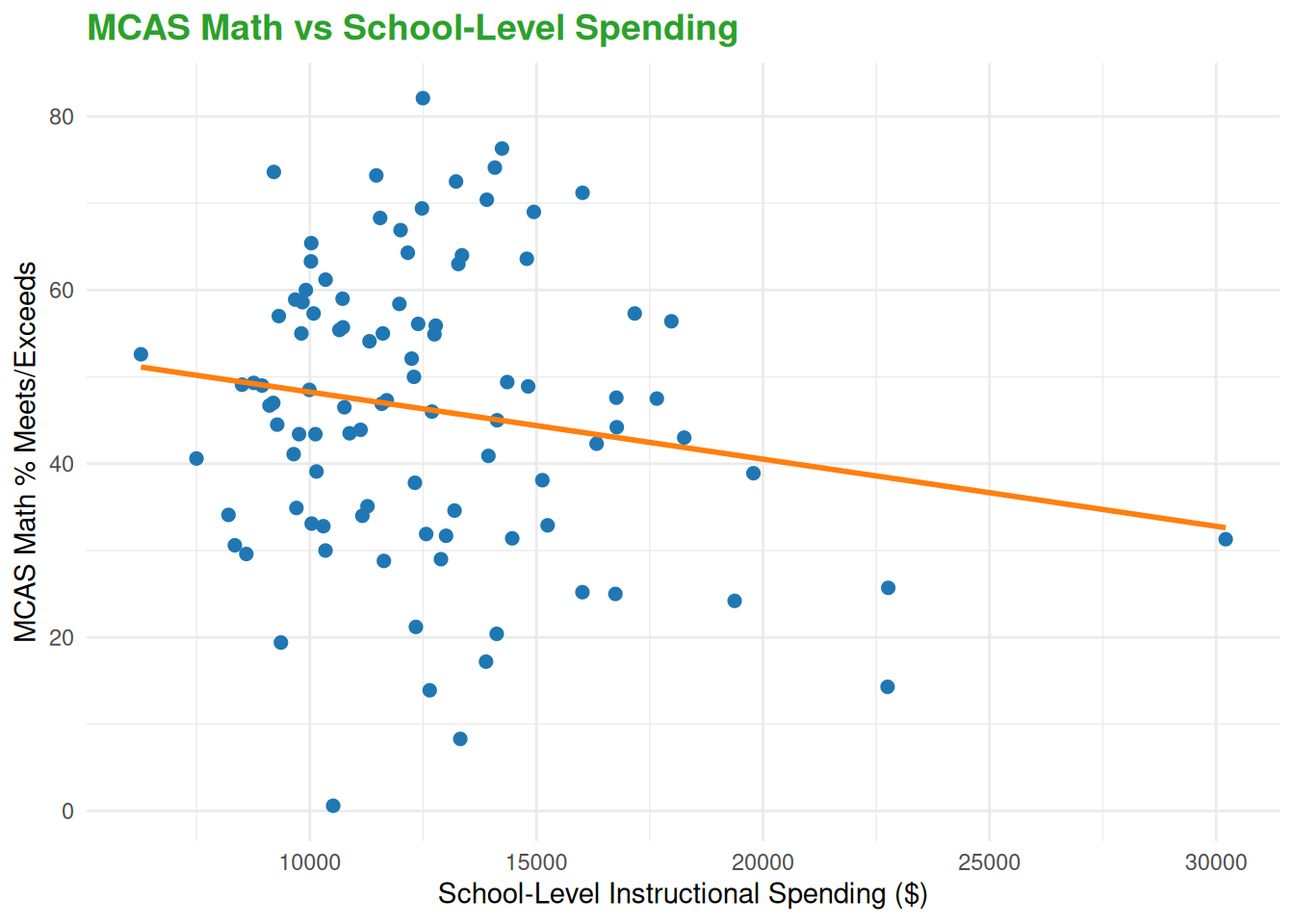
Each dollar spent in school-level instructional spending is associated with a 0.00115 percentage decease in the percentage of students in grades 3 to 8 that met or exceeds expectations on the MCAS Math examination, holding all other spending constant.

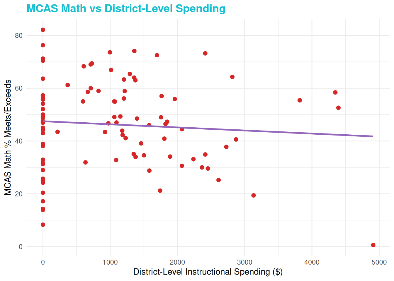
Each dollar spent in distinct level instructional expenditures is associated with a 0.00302 percentage decrease in the percentage of students in grades 3 to 8 that met or exceeds expectations on the MCAS Math examinations, holding all other spending constant.

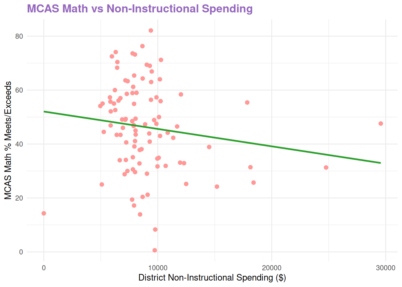
Each dollar spent in District Non-Instructional Expenditures is associated with a 0.0002 percentage decrease in the percentage of students in grades 3 to 8 that met or excceded expectations on the MCAS Math examinations, holding all other spending constant.

Questions of weither or not the pass rate is impacted by retakes (thus making it lower)

Plot:

library(ggplot2)

# Scatterplot: School-Level Instructional Spending
ggplot(analysis_df, aes(
  x = `School-Reported Instructional Expenditures`,
  y = `Math Grades 3-8 % Meets or Exceeds`
)) +
  geom_point(color = "#1f77b4", size = 2) +      # blue points
  geom_smooth(method = "lm", se = FALSE, color = "#ff7f0e") + # orange line
  labs(
    x = "School-Level Instructional Spending ($)",
    y = "MCAS Math % Meets/Exceeds",
    title = "MCAS Math vs School-Level Spending"
  ) +
  theme_minimal() +
  theme(plot.title = element_text(color = "#2ca02c", size = 14, face = "bold"))

# Scatterplot: District-Level Instructional Spending
ggplot(analysis_df, aes(
  x = `District-Level Instructional Expenditures`,
  y = `Math Grades 3-8 % Meets or Exceeds`
)) +
  geom_point(color = "#d62728", size = 2) +      # red points
  geom_smooth(method = "lm", se = FALSE, color = "#9467bd") + # purple line
  labs(
    x = "District-Level Instructional Spending ($)",
    y = "MCAS Math % Meets/Exceeds",
    title = "MCAS Math vs District-Level Spending"
  ) +
  theme_minimal() +
  theme(plot.title = element_text(color = "#17becf", size = 14, face = "bold"))

# Scatterplot: District Non-Instructional Spending
ggplot(analysis_df, aes(
  x = `District Non-Instructional Expenditures`,
  y = `Math Grades 3-8 % Meets or Exceeds`
)) +
  geom_point(color = "#ff9896", size = 2) +      # pink points
  geom_smooth(method = "lm", se = FALSE, color = "#2ca02c") + # green line
  labs(
    x = "District Non-Instructional Spending ($)",
    y = "MCAS Math % Meets/Exceeds",
    title = "MCAS Math vs Non-Instructional Spending"
  ) +
  theme_minimal() +
  theme(plot.title = element_text(color = "#9467bd", size = 14, face = "bold"))